Training deep learning models can be a pain. In particular, there is this perception that one of the reasons it's a pain is because you have to fiddle with learning rates. For example, arguably the most popular strategy for setting learning rates looks like this:
Run vanilla stochastic gradient descent with momentum and a fixed learning rate
Wait for the loss to stop improving
Reduce the learning rate
Go back to step 1 or stop if the learning rate is really small
Many papers reporting state-of-the-art results do this. There have been a lot of other methods proposed, like ADAM, but I've always found the above procedure to work best. This is a common finding. The only fiddly part of this procedure is the "wait for the loss to stop improving" step. A lot of people just eyeball a plot of the loss and manually intervene when it looks like its flattened out. Or worse, they pick a certain number of iterations ahead of time and blindly stop when that limit is reached. Both of these ways of deciding when to reduce the learning rate suck.
Fortunately, there is a simple method from classical statistics we can use to decide if the loss is still improving, and thus, when to reduce it. With this method it's trivial to fully automate the above procedure. In fact, it's what I've used to train all the public DNN models in dlib over the last few years: e.g. face detection, face recognition, vehicle detection, and imagenet classification. It's the default solving strategy used by dlib's DNN solver. The rest of this blog post explains how it works.
Fundamentally, what we need is a method that takes a noisy time series of $n$ loss values, $Y=\{y_0,y_1,y_2,\dots,y_{n-1}\}$, and tells us if the time series is trending down or not. To do this, we model the time series as a noisy line corrupted by Gaussian noise:
\[
\newcommand{\N} {\mathcal{N} } y_i = m\times i + b + \epsilon
\] Here, $m$ and $b$ are the unknown true slope and intercept parameters of the line, and $\epsilon$ is a Gaussian noise term with mean 0 and variance $\sigma^2$. Let's also define the function $\text{slope}(Y)$ that takes in a time series, performs OLS, and outputs the OLS estimate of $m$, the slope of the line. You can then ask the following question: what is the probability that a time series sampled from our noisy line model will have a negative slope according to OLS? That is, what is the value of?
\[
P(\text{slope}(Y) < 0)
\]If we could compute an estimate of $P(\text{slope}(Y)<0)$ we could use it to test if the loss is still decreasing. Fortunately, computing the above quantity turns out to be easy. In fact, $\text{slope}(Y)$ is a Gaussian random variable with this distribution:
\[
\text{slope}(Y) \sim \N\left(m, \frac{12 \sigma^2}{n^3-n}\right)
\]We don't know the true values of $m$ and $\sigma^2$, but they are easily estimated from data. We can obviously use $\text{slope}(Y)$ to estimate $m$. As for $\sigma^2$, it's customary to estimate it like this:
\[ \sigma^2 = \frac{1}{n-2} \sum_{i=0}^{n-1} (y_i - \hat y_i)^2 \] which gives an unbiased estimate of the true $\sigma^2$. Here $y_i - \hat y_i$ is the difference between the observed time series value at time $i$ and the value predicted by the OLS fitted line at time $i$. I should point out that none of this is new stuff, in fact, these properties of OLS are discussed in detail on the Wikipedia page about OLS.
So let's recap. We need a method to decide if the loss is trending downward or not. I'm suggesting that you use $P(\text{slope}(Y) < 0)$, the probability that a line fit to your loss curve will have negative slope. Moreover, as discussed above, this probability is easy to compute since it's just a question about a simple Gaussian variable and the two parameters of the Gaussian variable are given by a straightforward application of OLS.
You should also note that the variance of $\text{slope}(Y)$ decays at the very quick rate of $O(1/n^3)$, where $n$ is the number of loss samples. So it becomes very accurate as the length of the time series grows. To illustrate just how accurate this is, let's look at some examples. The figure below shows four different time series plots, each consisting of $n=4000$ points. Each plot is a draw from our noisy line model with parameters: $b=0$, $\sigma^2=1$, and $m \in \{0.001, 0.00004, -0.00004, -0.001\}$. For each of these noisy plots I've computed $P(\text{slope}(Y) < 0)$ and included it in the title.
From looking at these plots it should be obvious that $P(\text{slope}(Y) < 0)$ is quite good at detecting the slope. In particular, I doubt you can tell the difference between the two middle plots (the ones with slopes -0.00004 and 0.00004). But as you can see, the test statistic I'm suggesting, $P(\text{slope}(Y) < 0)$, has no trouble at all correctly identifying one as sloping up and the other as sloping down.
I find that a nice way to parameterize this in actual code is to count the number of mini-batches that executed while $P(\text{slope}(Y) < 0) < 0.51$. That is, find out how many loss values you have to look at before there is evidence the loss has been decreasing. To be very clear, this bit of pseudo-code implements the idea:
You can then use a rule like: "if the steps without decrease is 1000 I will lower the learning rate by 10x". However, there is one more issue that needs to be addressed. This is the fact that loss curves sometimes have really large transient spikes, where, for one reason or another (e.g. maybe a bad mini-batch) the loss will suddenly become huge for a moment. Not all models or datasets have this problem during training, but some do. In these cases, count_steps_without_decrease() might erroneously return a very large value. You can deal with this problem by discarding the top 10% of loss values inside count_steps_without_decrease(). This makes the entire procedure robust to these noisy outliers. Note, however, that the final test you would want to use is:
count_steps_without_decrease(Y) > threshold and count_steps_without_decrease_robust(Y) > threshold
That is, perform the check with and without outlier discarding. You need both checks because the 10% largest loss values might have occurred at the very beginning of Y. For example, maybe you are waiting for 1000 (i.e. threshold=1000) mini-batches to execute without showing evidence of the loss going down. And maybe the first 100 all showed a dropping loss while the last 900 were flat. The check that discarded the top 10% would erroneously indicate that the loss was NOT dropping. So you want to perform both checks and if both agree that the loss isn't dropping then you can be confident it's not dropping.
It should be emphasized that this method isn't substantively different from what a whole lot of people already do when training deep neural networks. The only difference here is that the "look at the loss and see if it's decreasing" step is being done by a computer. The point of this blog post is to point out that this check is trivially automatable with boring old simple statistics. There is no reason to do it by hand. Let the computer do it and find something more productive to do with your time than babysitting SGD. The test is simple to implement yourself, but if you want to just call a function you can call dlib's count_steps_without_decrease() and count_steps_without_decrease_robust() routines from C++ or Python.
Finally, one more useful thing you can do is the following: you can periodically check if $P(\text{slope}(Y) > 0) \gt 0.99$, that is, check if we are really certain that the loss is going up, rather than down. This can happen and I've had training runs that were going fine and then suddenly the loss shot up and stayed high for a really long time, basically ruining the training run. This doesn't seem to be too much of an issue with simple losses like the log-loss. However, structured loss functions that perform some kind of hard negative mining inside a mini-batch will sometimes go haywire if they hit a very bad mini-batch. You can fix this problem by simply reloading from an earlier network state before the loss increased. But to do this you need a reliable way to measure "the loss is going up" and $P(\text{slope}(Y) > 0) \gt 0.99$ is excellent for this task. This idea is called backtracking and has a long history in numerical optimization. Backtracking significantly increases solver robustness in many cases and is well worth using.
I get asked a lot of questions about dlib's landmarking tools. Some of the most common questions are about how to prepare a good training dataset. One of the most useful tricks for creating a dataset is to mirror the data, since this effectively doubles the amount of training data. However, if you do this naively you end up with a terrible training dataset that produces really awful landmarking models. Some of the most common questions I get are about why this is happening.
To understand the issue, consider the following image of an annotated face from the iBug W-300 dataset:
Since the mirror image of a face is still a face, we can mirror images like this to get more training data. However, what happens if you simply mirror the annotations? You end up with the wrong annotation labels! To see this, take a look at the figure below. The left image shows what happens if you naively mirror the above image and its landmarks. Note, for instance, that the points along the jawline are now annotated in reverse order. In fact, nearly all the annotations in the left image are wrong. Instead, you want to match the source image's labeling scheme. A mirrored image with the correct annotations is shown on the right.
Dlib's imglab tool has had a --flip option for a long time that would mirror a dataset for you. However, it used naive mirroring and it was left up to the user to adjust any landmark labels appropriately. Many users found this confusing, so in the new version of imglab (v1.13) the --flip command now performs automatic source label matching using a 2D point registration algorithm. That is, it left-right flips the dataset and annotations. Then it registers the mirrored landmarks with the original landmarks and transfers labels appropriately. In fact, the "source label matching" image on the right was created by the new version of imglab.
Finally, just to be clear, the point registration algorithm will work on anything. It doesn't have to be iBug's annotations. It doesn't have to be faces. It's a general point registration method that will work correctly for any kind of landmark annotated data with left-right symmetry. However, if you want the old --flip behavior you can use the new --flip-basic to get a naive mirroring. But most users will want to use the new --flip.
Here is a common problem: you have some machine learning algorithm you want to use but it has these damn hyperparameters. These are numbers like weight decay magnitude, Gaussian kernel width, and so forth. The algorithm doesn't set them, instead, it's up to you to determine their values. If you don't set these parameters to "good" values the algorithm doesn't work. So what do you do? Well, here is a list of everything I've seen people do, listed in order of most to least common:
Guess and Check: Listen to your gut, pick numbers that feel good and see if they work. Keep doing this until you are tired of doing it.
Grid Search: Ask your computer to try a bunch of values spread evenly over some range.
Random Search: Ask your computer to try a bunch of values by picking them randomly.
Bayesian Optimization: Use a tool like MATLAB's bayesopt to automatically pick the best parameters, then find out Bayesian Optimization has more hyperparameters than your machine learning algorithm, get frustrated, and go back to using guess and check or grid search.
Local Optimization With a Good Initial Guess: This is what MITIE does, it uses the BOBYQA algorithm with a well chosen starting point. Since BOBYQA only finds the nearest local optima the success of this method is heavily dependent on a good starting point. In MITIE's case we know a good starting point, but this isn't a general solution since usually you won't know a good starting point. On the plus side, this kind of method is extremely good at finding a local optima. I'll have more to say on this later.
The vast majority of people just do guess and check. That sucks and there should be something better. We all want some black-box optimization strategy like Bayesian optimization to be useful, but in my experience, if you don't set its hyperparameters to the right values it doesn't work as well as an expert doing guess and check. Everyone I know who has used Bayesian optimization has had the same experience. Ultimately, if I think I can do better hyperparameter selection manually then that's what I'm going to do, and most of my colleagues feel the same way. The end result is that I don't use automated hyperparameter selection tools most of the time, and that bums me out. I badly want a parameter-free global optimizer that I can trust to do hyperparameter selection.
So I was very excited when I encountered the paper Global optimization of Lipschitz functions by Cédric Malherbe and Nicolas Vayatis in this year's international conference on machine learning. In this paper, they propose a very simple parameter-free and provably correct method for finding the $x \in \mathbb{R}^d$ that maximizes a function, $f(x)$, even if $f(x)$ has many local maxima. The key idea in their paper is to maintain a piecewise linear upper bound of $f(x)$ and use that to decide which $x$ to evaluate at each step of the optimization. So if you already evaluated the points $x_1, x_2, \cdots, x_t$ then you can define a simple upper bound on $f(x)$ like this:
\[ \newcommand{\norm}[1]{\left\lVert#1\right\rVert} U(x) = \min_{i=1\dots t} (f(x_i) + k \cdot \norm{x-x_i}_2 ) \] Where $k$ is the Lipschitz constant for $f(x)$. Therefore, it is trivially true that $U(x) \geq f(x), \forall x$, by the definition of the Lipschitz constant. The authors go on to suggest a simple algorithm, called LIPO, that picks points at random, checks if the upper bound for the new point is better than the best point seen so far, and if so selects it as the next point to evaluate. For example, the figure below shows a plot of a simple $f(x)$ in red with a plot of its associated upper bound $U(x)$ in green. In this case $U(x)$ is defined by 4 points, indicated here with little black squares.
It shouldn't take a lot of imagination to see how the upper bound helps you pick good points to evaluate. For instance, if you selected the max upper bound as the next iterate you would already get pretty close to the global maximizer. The authors go on to prove a bunch of nice properties of this method. In particular, they both prove mathematically and show empirically that the method is better than random search in a number of non-trivial situations. This is a fairly strong statement considering how competitive random hyperparameter search turns out to be relative to competing hyperparameter optimization methods. They also compare the method to other algorithms like Bayesian optimization and show that it's competitive.
But you are probably thinking: "Hold on a second, we don't know the value of the Lipschitz constant $k$!". This isn't a big deal since it's easily estimated, for instance, by setting $k$ to the largest observed slope of $f(x)$ before each iteration. That's equivalent to solving the following easy problem:
\begin{align}
\min_{k} & \quad k^2 \\
\text{s.t.} & \quad U(x_i) \geq f(x_i), \quad \forall i \in [1\dots t] \\
& \quad k \geq 0
\end{align} Malherbe et al. test a variant of this $k$ estimation approach and show it works well.
This is great. I love this paper. It's proposing a global optimization method called LIPO that is both parameter free and provably better than random search. It's also really simple. Reading this paper gives you one of those "duah" moments where you wonder why you didn't think of this a long time ago. That's the mark of a great paper. So obviously I was going to add some kind of LIPO algorithm to dlib, which I did in the recent dlib v19.8 release.
However, if you want to use LIPO in practice there are some issues that need to be addressed. The rest of this blog post discusses these issues and how the dlib implementation addresses them. First, if $f(x)$ is noisy or discontinuous even a little it's not going to work reliably since $k$ will be infinity. This happens in real world situations all the time. For instance, evaluating a binary classifier against the 0-1 loss gives you an objective function with little discontinuities anywhere samples switch their predicted class. You could cross your fingers and run LIPO anyway, but you run the very real risk of two $x$ samples closely straddling a discontinuity and causing the estimated $k$ to explode. Second, not all hyperparameters are equally important, some hardly matter while small changes in others drastically affect the output of $f(x)$. So it would be nice if each hyperparameter got its own $k$. You can address these problems by defining the upper bound $U(x)$ as follows:
\[ U(x) = \min_{i=1\dots t} \left[ f(x_i) + \sqrt{\sigma_i +(x-x_i)^\intercal K (x-x_i)} \ \right] \] Now each sample from $f(x)$ has its own noise term, $\sigma_i$, which should be 0 most of the time unless $x_i$ is really close to a discontinuity or there is some stochasticity. Here, $K$ is a diagonal matrix that contains our "per hyperparameter Lipschitz $k$ terms". With this formulation, setting each $\sigma$ to 0 and $K=k^2I$ gives the same $U(x)$ as suggested by Malherbe et al., but if we let them take more general values we can deal with the above mentioned problems.
Just like before, we can find the parameters of $U(x)$ by solving an optimization problem:
\begin{align}
\min_{K,\sigma} & \quad \norm{K}^2_F + 10^6 \sum_{i=1}^t {\sigma_i^2} &\\
\text{s.t.} & \quad U(x_i) \geq f(x_i), & \quad \forall i \in [1\dots t] \\
& \quad \sigma_i \geq 0 & \quad \forall i \in [1\dots t] \\
& \quad K_{i,j} \geq 0 & \quad \forall i,j \in [1\dots d] \\
& \quad \text{K is a diagonal matrix}
\end{align} The $10^6$ penalty on $\sigma^2$ causes most $\sigma$ terms to be exactly 0. The behavior of the whole algorithm is insensitive to the particular penalty value used here, so long as it's reasonably large the $\sigma$ values will be 0 most of the time while still preventing $k$ from becoming infinite, which is the behavior we want. It's also possible to rewrite this as a big quadratic programming problem and solve it with a dual coordinate descent method. I'm not going into the details here. It's all in the dlib code for those really interested. The TL;DR is that it turns out to be easy to solve using well known methods and it fixes the infinite $k$ problem.
The final issue that needs to be addressed is LIPO's terrible convergence in the area of a local maximizer. So while it's true that LIPO is great at getting onto the tallest peak of $f(x)$, once you are there it does not make very rapid progress towards the optimal location (i.e. the very top of the peak). This is a problem shared by many derivative free optimization algorithms, including MATLAB's Bayesian optimization tool. Fortunately, not all methods have this limitation. In particular, the late and great Michael J. D. Powell wrote a series of papers on how to apply classic trust region methods to derivative free optimization. These methods fit a quadratic surface around the best point seen so far and then take the next iterate to be the maximizer of that quadratic surface within some distance of the current best point. So we "trust" this local quadratic model to be accurate within some small region around the best point, hence the name "trust region". The BOBYQA method I mentioned above is one of these methods and it has excellent convergence to the nearest local optima, easily finding local optima to full floating point precision in a very small number of steps.
We can fix LIPO's convergence problem by combining these two methods, LIPO will explore $f(x)$ and quickly find a point on the biggest peak. Then a Powell style trust region method can efficiently find the exact maximizer of that peak. The simplest way to combine these two things is to alternate between them, which is what dlib does. On even iterations we pick the next $x$ according to our upper bound while on odd iterations we pick the next $x$ according to the trust region model. I've also used a slightly different version of LIPO that I'm calling MaxLIPO. Recall that Malherbe et al. suggest selecting any point with an upper bound larger than the current best objective value. However, I've found that selecting the maximum upper bounding point on each iteration is slightly better. This alternative version, MaxLIPO, is therefore what dlib uses. You can see this hybrid of MaxLIPO and a trust region method in action in the following video:
In the video, the red line is the function to be optimized and we are looking for the maximum point. Every time the algorithm samples a point from the function we note it with a little box. The state of the solver is determined by the global upper bound $U(x)$ and the local quadratic model used by the trust region method. Therefore, we draw the upper bounding model as well as the current local quadratic model so you can see how they evolve as the optimization proceeds. We also note the location of the best point seen so far by a little vertical line.
You can see that the optimizer is alternating between picking the maximum upper bounding point and the maximum point according to the quadratic model. As the optimization proceeds, the upper bound becomes progressively more accurate, helping to find the best peak to investigate, while the quadratic model quickly finds a high precision maximizer on whatever peak it currently rests. These two things together allow the optimizer to find the true global maximizer to high precision (within $\pm{10^{-9}}$ in this case) by the time the video concludes.
The Holder Table Test Function from https://en.wikipedia.org/wiki/File:Holder_table_function.pdf
Now let's do an experiment to see how this hybrid of MaxLIPO and Powell's trust region method (TR) compares to MATLAB's Bayesian optimization tool with its default settings. I ran both algorithms on the Holder table test function 100 times and plotted the average error with one standard deviation error bars. So the plot below shows $f(x^\star)-f(x_i)$, the difference between the true global optimum and the best solution found so far, as a function of the number of calls to $f(x)$. You can see that MATLAB's BayesOpt stalls out at an accuracy of about $\pm{10^{-3}}$ while our hybrid method (MaxLIPO+TR, the new method in dlib) quickly approaches full floating point precision of around $\pm{10^{-17}}$.
I also reran some of the tests from Figure 5 of the LIPO paper. The results are shown in the table below. In these experiments I compared the performance of LIPO with and without the trust region solver (LIPO+TR and LIPO). Additionally, to verify that LIPO is better than pure random search I tested a version of the algorithm that alternates between pure random search and the trust region solver (PRS+TR) rather than alternating between a LIPO method and a trust region solver (LIPO+TR and MaxLIPO+TR). Pure random search (PRS) is also included for reference. Finally, the new algorithm implemented in dlib, MaxLIPO+TR, is included as well. In each test I ran the algorithm 1000 times and recorded the mean and standard deviation of the number of calls to $f(x)$ required to reach a particular solution accuracy. For instance, $\epsilon=0.01$ means that $f(x^\star)-f(x_i) \leq 0.01$, while "target 99%" uses the "target" metric from Malherbe's paper, which for most tests corresponds to an $\epsilon > 0.1$. Tests that took too long to execute are noted with a - symbol.
The key points to notice about these results are that the addition of a trust region method allows LIPO to reach much higher solution accuracy. It also makes the algorithm run faster. Recall that LIPO works internally by using random search of $U(x)$. Therefore, the number of calls LIPO makes to $U(x)$ is at least as many as PRS would require when searching $f(x)$. So for smaller $\epsilon$ it becomes very expensive to execute LIPO. For instance, I wasn't able to get results for LIPO, by itself, at accuracies better than $0.1$ on any of the test problems since it took too long to execute. However, with a trust region method the combined algorithm can easily achieve high precision solutions. The other significant detail is that, for tests with many local optima, all methods combining LIPO with TR are much better than PRS+TR. This is most striking on ComplexHolder, which is a version of the HolderTable test function with additional high frequency sinusoidal noise that significantly increases the number of local optima. On ComplexHolder, LIPO based methods require about an order of magnitude fewer calls to $f(x)$ than PRS+TR, further justifying the claims by Malherbe et al. of the superiority of LIPO relative to pure random search.
The new method in dlib, MaxLIPO+TR, fares the best in all my tests. What is remarkable about this method is its simplicity. In particular, MaxLIPO+TR doesn't have any hyperparameters, making it very easy to use. I've been using it for a while now for hyperparameter optimization and have been very pleased. It's the first black-box hyperparameter optimization algorithm I've had enough confidence in to use on real problems.
Finally, here is an example of how you can use this new optimizer from Python:
defholder_table(x0,x1):return-abs(sin(x0)*cos(x1)*exp(abs(1-sqrt(x0*x0+x1*x1)/pi)))x,y=dlib.find_min_global(holder_table,[-10,-10],# Lower bound constraints on x0 and x1 respectively[10,10],# Upper bound constraints on x0 and x1 respectively80)# The number of times find_min_global() will call holder_table()
Or in C++11:
auto holder_table = [](double x0, double x1){return-abs(sin(x0)*cos(x1)*exp(abs(1-sqrt(x0*x0+x1*x1)/pi)));};
// obtain result.x and result.y
auto result =find_min_global(holder_table,
{-10,-10}, // lower bounds
{10,10}, // upper bounds
max_function_calls(80));
Both of these methods find holder_table's global optima to about 12 digits of precision in about 0.1 seconds. The C++ API exposes a wide range of ways to call the solver, including optimizing multiple functions at a time and adding integer constraints. See the documentation for full details.
Dlib 19.8 is officially out. There are a lot of changes, but the two most interesting ones are probably the new global optimizer and semantic segmentation examples. The global optimizer is definitely my favorite as it allows you to easily find the optimal hyperparameters for machine learning algorithms. It also has a very convenient syntax. For example, consider the Holder table test function:
From https://en.wikipedia.org/wiki/File:Holder_table_function.pdf
Here is how you could use dlib's new optimizer from Python to optimize the difficult Holder table function:
defholder_table(x0,x1):return-abs(sin(x0)*cos(x1)*exp(abs(1-sqrt(x0*x0+x1*x1)/pi)))x,y=dlib.find_min_global(holder_table,[-10,-10],# Lower bound constraints on x0 and x1 respectively[10,10],# Upper bound constraints on x0 and x1 respectively80)# The number of times find_min_global() will call holder_table()
Or in C++:
auto holder_table = [](double x0, double x1){return-abs(sin(x0)*cos(x1)*exp(abs(1-sqrt(x0*x0+x1*x1)/pi)));};
// obtain result.x and result.y
auto result =find_min_global(holder_table,
{-10,-10}, // lower bounds
{10,10}, // upper bounds
max_function_calls(80));
Both of these methods find holder_table's global optima to about 12 digits of precision in about 0.1 seconds. The documentation has much more to say about this new tooling. I'll also make a blog post soon that goes into much more detail on how the method works.
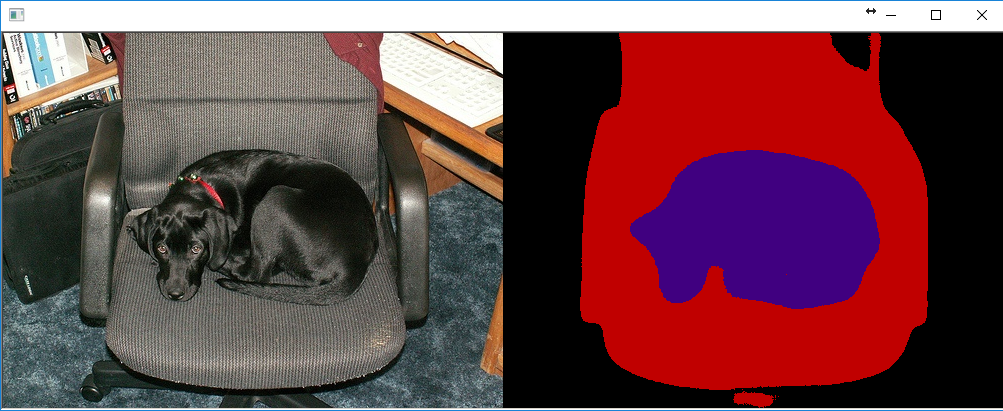
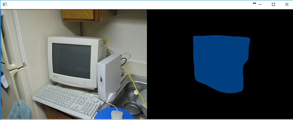
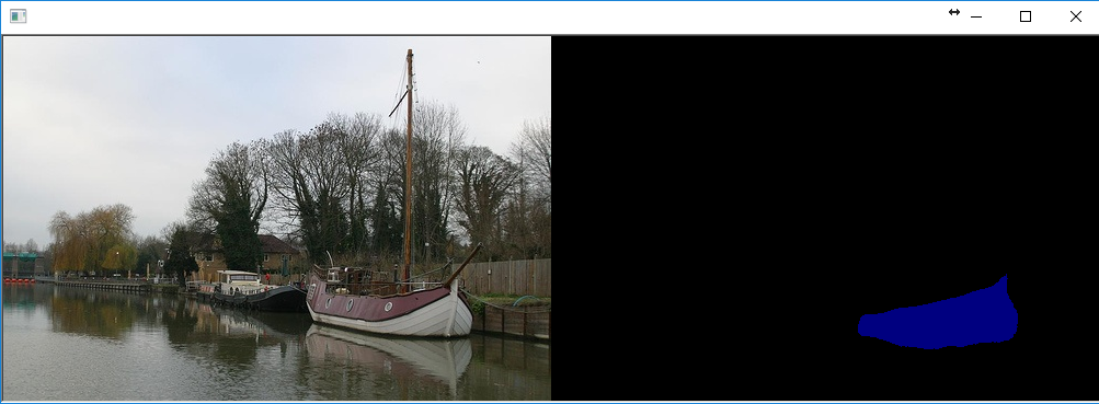
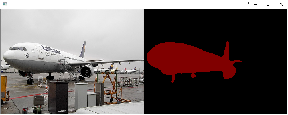
Finally, here are some fun example outputs from the new semantic segmentation example program:
The new version of dlib is out and the biggest new feature is the ability to train multiclass object detectors with dlib's convolutional neural network tooling. The previous version only allowed you to train single class detectors, but this release adds the option to create single CNN models that output multiple labels. As an example, I created a small 894 image dataset where I annotated the fronts and rears of cars and used it to train a 2-class detector. You can see the resulting detector running in this video:
If you want to run the car detector from this video on your own images you can check out this example program.
I've also improved the detector speed in dlib 19.7 by pushing more of the processing to the GPU. This makes the detector 2.5x faster. For example, running the detector on the 928x478 image used in this example program ran at 39fps in the previous version of dlib, but now runs at 98fps (when run on a NVIDIA 1080ti).
This release also includes a new 5-point face landmarking model that finds the corners of the eyes and bottom of nose:
Unlike the 68-point landmarking model included with dlib, this model is over 10x smaller at 8.8MB compared to the 68-point model's 96MB. It also runs faster, and even more importantly, works with the state-of-the-art CNN face detector in dlib as well as the older HOG face detector in dlib. The central use-case of the 5-point model is to perform 2D face alignment for applications like face recognition. In any of the dlib code that does face alignment, the new 5-point model is a drop-in replacement for the 68-point model and in fact is the new recommended model to use with dlib's face recognition tooling.
Dlib v19.5 is out and there are a lot of new features. There is a dlib to caffe converter, a bunch of new deep learning layer types, cuDNN v6 and v7 support, and a bunch of optimizations that make things run faster in different situations, like ARM NEON support, which makes HOG based detectors run a lot faster on mobile devices.
However, the coolest and most requested feature has been an upgrade to the CNN+MMOD object detector to support detecting things with varying aspect ratios. The previous version of the detector required the training data to consist of objects that all had essentially the same aspect ratio. This is fine for tasks like face detection and dog hipsterization, but obviously not as general as you would like.
So dlib v19.5 includes an updated version of the MMOD loss layer that can be used to learn an object detector from a dataset with any mixture of bounding box shapes and sizes. To demo this new feature, I used the new MMOD code to create a vehicle detector, which you can see running on these videos. This detector is trained to find cars moving with you in traffic, and therefore cars where the rear end of the vehicle is visible.
The detector is just as fast as previous versions of the CNN+MMOD detector. For instance, when I run it on my NVIDIA 1080ti I can process 39 frames per second when processing them individually and 93 frames per second when processing them grouped into batches. This assumes a frame size of 928x478.
If you want to run this detector yourself you can check out the new example program that does just that. The detector was trained on a modest dataset of 2217 images, which is also available, as is the training code. Both these new example programs contain a lot of information about training this kind of detector and are worth reading if you want to understand the details involved. However, we can go into a short description here to understand how the detector works.
Take this image as an example. I ran the new vehicle detector on it and plotted the resulting detections as red boxes. So what are the processing steps that go from the raw image to the 6 boxes? To roughly summarize, they are:
Create an image pyramid and pack the pyramid into one big image. Let's call this the "tiled pyramid"
Run the tiled pyramid image through a CNN. The CNN outputs a new image where bright pixels in the output image indicate the presence of cars.
Find pixels in the CNN's output image with a value > 0. Those locations are your preliminary car detections.
Perform non-maximum suppression on the preliminary detections to produce the final output.
Steps 3 and 4 are pretty straightforward. It's the first two steps that are complicated. So to understand them, let's visualize the outputs of these first two steps. All step 1 does is call dlib::create_tiled_pyramid on the input image to produce this new image:
What's special about this image is that we don't need to worry about scale anymore. That is, suppose we have a detection algorithm that can find cars, but it only knows how to find cars of a certain size. No problem. When you run it on this tiled pyramid image you are going to find each car somewhere in it at the scale your detector expects. Moreover, the tiled pyramid is only about 3.7 times larger than the original image, so processing it instead of the raw image gives us full scale invariance for only a 3.7x increase in computational cost. That's a very reasonable trade. Moreover, tiling it inside a rectangular image makes it very easy to process using normal CNN tooling on a GPU and still get full GPU speeds.
Now for step 2. The CNN takes the tiled pyramid as input, does a bunch of convolutions, and outputs a new set of images. In the case of our vehicle detector, it outputs 3 new images, each is a detection strength map that gets "hot" in locations likely to contain a vehicle. The reason there are 3 images for the vehicle detector is because there are, roughly, 3 different aspect ratios (tall and skinny e.g. semi trucks, short and wide e.g. sedans, and squarish e.g. SUVs). For purposes of display, I have combined the 3 images into one by taking the pointwise max of the 3 original images. You can see this combined image below. The dark blue areas are places the CNN is saying "definitely not a vehicle" and the bright red locations are the positions it thinks contain a vehicle.
If we overlay this CNN output on top of the tiled pyramid you can see it's doing the right thing. The cars get bright red dots on them, right in the centers of the cars. Moreover, you can tell that the CNN is only detecting cars at a certain scale. The smaller cars are detected at the top of the pyramid and only as we progress down the pyramid does it begin to detect the larger cars.
After the CNN output is obtained, all the detection code needs to do is threshold the CNN output, find all the hot spots, apply non-max suppression, and output the boxes corresponding to the identified hot spots. And that's it, that's all the CNN+MMOD detector is doing.
On the other hand, describing how the CNN is trained is more complicated. The code in dlib uses the usual stochastic gradient descent methods. You can see many of the details if you read the dlib DNN example programs. How deep learning works in general is a big topic, but the thing most interesting here is the MMOD loss layer. For the gory details on that I refer you to the MMOD paper which explains the loss function. In the paper it is discussed in the context of networks that are linear in their parameters rather than non-linear in their parameters, as is our CNN here. However, for understanding the loss the difference between linear vs. non-linear is a minor detail. In fact, the loss equations are the same for both cases. The only difference is what kind of optimization algorithms are available for each case. In the linear parameter case you can write a fancy numeric solver capable of solving the problem in a few minutes, but with a non-linear parameterization you have to resort to brute force SGD and GPUs running for many hours.
But at a very high level, it's running the entire detection process over and over during training, counting the number of detection mistakes (false alarms, missed detections, and duplicate detections), and back-propagating that error gradient through the CNN until the CNN stops messing up. Also, since the MMOD loss layer is counting mistakes after non-max suppression is applied, it knows that it needs to get the CNN to avoid producing high outputs in parts of the image that won't be suppressed by non-max suppression. This is why you see the dark blue areas of "definitely not a car" surrounding each of the car detections. The CNN has learned that it needs to be very careful on the border between "it's a car" and "it's not a car" to avoid accidentally detecting the same car multiple times.
This is perhaps easiest to see if we merge the pyramid layers back into the original image. If we make an image where the pixel value is the max over all scales in the pyramid we get this image:
Here you can clearly see the 6 car hotspots and the dark blue areas of "not a car" immediately surrounding them. Finally, overlaying this on the original image gives this wonderful image:
Since the last dlib release, I've been working on adding easy to use deep metric learning tooling to dlib. Deep metric learning is useful for a lot of things, but the most popular application is face recognition. So obviously I had to add a face recognition example program to dlib. The new example comes with pictures of bald Hollywood action heroes and uses the provided deep metric model to identify how many different people there are and which faces belong to each person. The input images are shown below along with the four automatically identified face clusters:
Just like all the other example dlib models, the pretrained model used by this example program is in the public domain. So you can use it for anything you want. Also, the model has an accuracy of 99.38% on the standard Labeled Faces in the Wild benchmark. This is comparable to other state-of-the-art models and means that, given two face images, it correctly predicts if the images are of the same person 99.38% of the time.
For those interested in the model details, this model is a ResNet network with 29 conv layers. It's essentially a version of the ResNet-34 network from the paper Deep Residual Learning for Image Recognition by He, Zhang, Ren, and Sun with a few layers removed and the number of filters per layer reduced by half.
The network was trained from scratch on a dataset of about 3 million faces. This dataset is derived from a number of datasets. The face scrub dataset[2], the VGG dataset[1], and then a large number of images I personally scraped from the internet. I tried as best I could to clean up the combined dataset by removing labeling errors, which meant filtering out a lot of stuff from VGG. I did this by repeatedly training a face recognition model and then using graph clustering methods and a lot of manual review to clean up the dataset. In the end, about half the images are from VGG and face scrub. Also, the total number of individual identities in the dataset is 7485. I made sure to avoid overlap with identities in LFW so the LFW evaluation would be valid.
The network training started with randomly initialized weights and used a structured metric loss that tries to project all the identities into non-overlapping balls of radius 0.6. The loss is basically a type of pair-wise hinge loss that runs over all pairs in a mini-batch and includes hard-negative mining at the mini-batch level. The training code is obviously also available, since that sort of thing is basically the point of dlib. You can find all details on training and model specifics by reading the example program and consulting the referenced parts of dlib. There is also a Python API for accessing the face recognition model.
[1] O. M. Parkhi, A. Vedaldi, A. Zisserman Deep Face Recognition British Machine Vision Conference, 2015.
[2] H.-W. Ng, S. Winkler. A data-driven approach to cleaning large face datasets. Proc. IEEE International Conference on Image Processing (ICIP), Paris, France, Oct. 27-30, 2014